Simple Dynamic Segment - v3
This example pulls the top 10 pages for the last thirty days, for visits that occurred on a mobile device. We’ll doing this by defining a dynamic segment using the v3 (older) version of the Google Analytics API. This returns the exact same results as these two examples, but through different means for defining/referencing the segment:
- Simple Dynamic Segment - v4 – defining the segment using the v4 API syntax (which is super-cumbersome for a super simple segment like this one, but illustrative nonetheless)
- Apply Segment by Segment ID – simply using the ID of either a standard segment or a custom segment built in the Google Analytics web interface
All three approaches are perfectly acceptable.
Setup/Config
Be sure you’ve completed the steps on the Initial Setup page before running this code.
For the setup, we’re going to load a few libraries, load our specific Google Analytics credentials, and then authorize with Google.
# Load the necessary libraries. These libraries aren't all necessarily required for every
# example, but, for simplicity's sake, we're going ahead and including them in every example.
# The "typical" way to load these is simply with "library([package name])." But, the handy
# thing about using the approach below -- which uses the pacman package -- is that it will
# check that each package exists and actually install any that are missing before loading
# the package.
if (!require("pacman")) install.packages("pacman")
pacman::p_load(googleAnalyticsR,  # How we actually get the Google Analytics data
               tidyverse,         # Includes dplyr, ggplot2, and others; very key!
               devtools,          # Generally handy
               googleVis,         # Useful for some of the visualizations
               scales)            # Useful for some number formatting in the visualizations

# Authorize GA. Depending on if you've done this already and a .ga-httr-oauth file has
# been saved or not, this may pop you over to a browser to authenticate.
ga_auth(token = ".ga-httr-oauth")

# Set the view ID and the date range. If you want to, you can swap out the Sys.getenv()
# call and just replace that with a hardcoded value for the view ID. And, the start
# and end date are currently set to choose the last 30 days, but those can be
# hardcoded as well.
view_id <- Sys.getenv("GA_VIEW_ID")
start_date <- Sys.Date() - 31        # 30 days back from yesterday
end_date <- Sys.Date() - 1           # Yesterday
If that all runs with just some messages but no errors, then you’re set for the next chunk of code: pulling the data.
Pull the Data
The trick to this is that we actually pass the v3 dynamic segment definition into the segment_id argument for segment_ga4(). It’s not super-intuitive, because we’re passing the actual segment definition rather than an “id”… but when cramming v3 stuff into a v4 world, we’ve got to be a little forgiving, no?
# For code readability, create a separate object with the segment definition.
mobile_segment_v3 <- "sessions::condition::ga:deviceCategory==Mobile"

# Create the segment object. See ?segment_ga4() for details. Note that, it doesn't
# really matter what we put for the name argument -- because this is pulling a v3
# dynamic segment, the name that appears in the output is just "Dynamic Segment."
my_segment <- segment_ga4("Mobile Sessions Only",
                          segment_id = mobile_segment_v3)

# Pull the data. See ?google_analytics_4() for additional parameters. Depending on what
# you're expecting back, you probably would want to use an "order" argument to get the
# results in descending order. But, we're keeping this example simple. Note, though, that
# we're still wrapping my_segment in a list() (of one element).
ga_data <- google_analytics(viewId = view_id,
                              date_range = c(start_date, end_date),
                              metrics = "pageviews",
                              dimensions = "pagePath",
                              segments = my_segment)

# Go ahead and do a quick inspection of the data that was returned. This isn't required,
# but it's a good check along the way.
head(ga_data)| pagePath | segment | pageviews |
|---|---|---|
| / | Dynamic Segment | 269 |
| /?__hstc=205162639.2492ee4e2514a59ed226f9dc5224e8b6.1537248787762.1537248787762.1537248787762.1&__hssc=205162639.1.1537248787763&__hsfp=2964561211&hsCtaTracking=8bc9e3c4-0d81-453f-9aa0-e7ee2d150e86|4361a058-c61b-4634-98be-95a3d7d9cb0c | Dynamic Segment | 1 |
| /?__hstc=205162639.3ee49b04f9a3ca95eff26980d8739ac8.1537165640249.1537165640249.1537165640249.1&__hssc=&hsCtaTracking=8bc9e3c4-0d81-453f-9aa0-e7ee2d150e86|4361a058-c61b-4634-98be-95a3d7d9cb0c | Dynamic Segment | 1 |
| /about/ | Dynamic Segment | 43 |
| /about/career-spotlights/ | Dynamic Segment | 1 |
| /about/careers/ | Dynamic Segment | 83 |
Data Munging
Since we didn’t sort the data when we queried it, let’s go ahead and sort it here and grab just the top 10 pages.
# Using dplyr, sort descending and then grab the top 10 values. We also need to make the
# page column a factor so that the order will be what we want when we chart the data.
# This is a nuisance, but you get used to it. That's what the mutate function is doing
ga_data_top_10 <- ga_data %>%
  arrange(-pageviews) %>%
  top_n(10) %>%
  mutate(pagePath = factor(pagePath,
                           levels = rev(pagePath)))

# Take a quick look at the result.
head(ga_data_top_10)| pagePath | segment | pageviews |
|---|---|---|
| / | Dynamic Segment | 269 |
| /open-positions/ | Dynamic Segment | 124 |
| /about/careers/ | Dynamic Segment | 83 |
| /solutions/industries/ | Dynamic Segment | 49 |
| /solutions/partners/adobe/adobe-launch/dtm-launch-assessment/ | Dynamic Segment | 48 |
| /about/ | Dynamic Segment | 43 |
Data Visualization
This won’t be the prettiest bar chart, but let’s make a horizontal bar chart with the data. Remember, in ggplot2, a horizontal bar chart is just a normal bar chart with coord_flip().
# Create the plot. Note the stat="identity"" (because the data is already aggregated) and
# the coord_flip(). And, I just can't stand it... added on the additional theme stuff to
# clean up the plot a bit more.
gg <- ggplot(ga_data_top_10, mapping = aes(x = pagePath, y = pageviews)) +
  geom_bar(stat = "identity") +
  coord_flip() +
  theme_light() +
  theme(panel.grid.major.y = element_blank(),
        panel.grid.minor.y = element_blank(),
        panel.border = element_blank(),
        axis.title.y = element_blank(),
        axis.ticks.y = element_blank())

# Output the plot. You *could* just remove the "gg <-" in the code above, but it's
# generally a best practice to create a plot object and then output it, rather than
# outputting it on the fly.
gg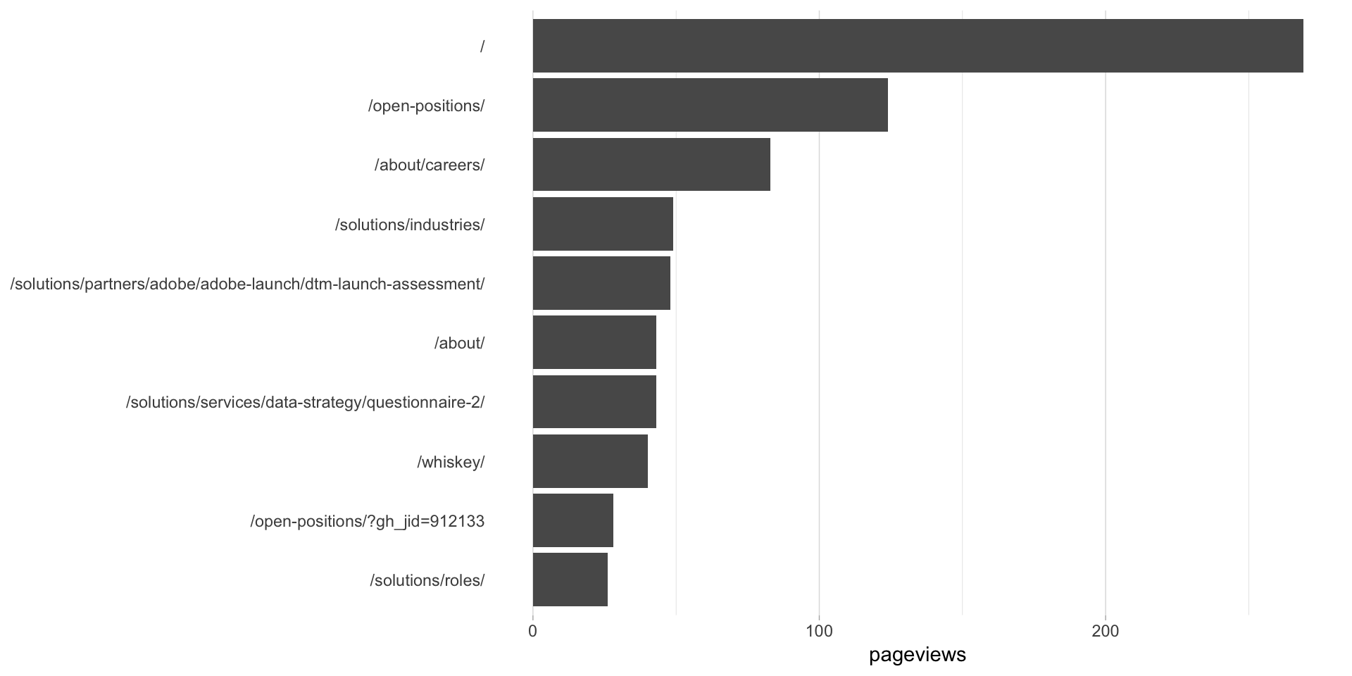
This site is a sub-site to dartistics.com