Regression
Regression is a way to represent cause and effect between two (or more variables). It attempts to make a best guess or model on how variables influence each other, and gives you an equation which you can use to predict future values.
If you want to just measure how closely two variables are and in which direction, correlation is more appropriate. However, if you want to try and make predictions from another metric then regression may be the tool for you.
Regression allows us to determine what independent variable, or variables, predict a dependent variable. In it is simplest form, one independent variable that is metric in nature predicts one dependent variable that is metric in nature. This form of regression is referred to as bivariate regression.
If we add one or more independent variable that are metric in nature, then we are working with multiple regression.
Note: In regression, the independent variable is noted by an \(x\). The dependent variable is noted by a \(y\).
Correspondingly, bivariate regression and 1-way ANOVA appear similar in that both included one independent variable while N-way ANOVA and multiple variable regression have two or more \(X\)s. However, in ANOVA, the independent variable is nominal. In regression, the independent variable is interval or ratio.
Regression Question
A digital analyst could ask, “Does unique visitors predict number of goals completed?”
Unique visitors would be the independent variable that would predict the number of goals completed, which is the dependent variable.
Regression Answer
To answer this question, start with a scatter plot of each X on the horizontal axis and Y on the vertical axis. The scatter plot will provide some insight into the relationship between each X and the Y variables. Regardless of the shape and direction of the scatter plot, a line can be fitted through it to establish a relationship.
This line is determined by regression.
Mathematically, we write the simple linear regression model:
\[Y = B_0 + B_1X + \epsilon\]
This equation appears similar to the equation of a line learned in high school geometry class:
\[y = mx + b\]
Here, \(B_0\) (or \(b\)) represents the y-intercept. \(B_1\) (or \(m\)) represents the slope. In bivariate regression, the interpretation of \(B_0\) and \(B_1\) will differ from \(b\) and \(m\), respectively.
As the \(y\)-intercept, \(B_0\) is interpreted as, if we do not increase or decrease the independent variable, then we would expect some number, \(Y\).
As the slope, \(B_1\) is interpreted as, if we increase \(X\) by 1 unit, then we should expect a \(B_1\) increase in \(Y\).
Epsilon (\(\epsilon\)) represents the residual, or the left over, values that were not included in our equation. As the residual decreases, then our regression model (or line) includes fundamental or key independent variables. Conversely, as the residual increases, then our regression model (or line) excludes fundamental or key independent variables.
For example, a digital analyst performs a regression analysis (after taking this workshop) and finds this equation:
\(Y = 100 + 50_x\) where \(Y\) represents the number of goals completed and \(X\) is the number of unique visitors. If a website receives no changes in the number of unique visitors, then we would expect 100 completed goals. If we add one more unique visitor, then we expect 50 more completed goals.
By adding more variables, the equation of the line can be extended to:
\[Y = B_0 + B_1X_1 + B_2X_2 + … + B_nX_n\]
Later, in this document, we will discuss how to include nominal variables in both the dependent variable and independent variable.
Put on the Hat
A detour here: \(Y = B_0 + B_1X_1\) represents the estimated line. When we run a regression analysis, then we are generating a predicted line. The notation changes slightly. Instead of using \(Y\), we use \(\hat{Y}\) (pronounced “Y-hat”). So, the line changes notation to \(\hat{Y} = b_0 + b_1x_1\).
Depending on the book and/or the instructor, \(b_0\) is also expressed as a lowercase \(a\). Regardless of notation, \(b_0\) or \(a\), refers to the \(y\)-intercept.
The error that we are interested appears in the dependent variable, or \(Y\). Specifically, we are interested in the error, or distance, from the observed \(Y\) and the predicted \(Y\), \(\hat{Y}\).
Some Basic Math to Link to ANOVA
If I square that error (\(\hat{Y} - Y\)), then I have squared the error.
If I sum all the square errors, then I have determined the sum of square error. Yes, the same sum of square error (\(SS_E\)) from ANOVA!
Recall from ANOVA: I wanted to decompose or divide the sum of square error (\(SS_y\)) in the levels of the dependent variable. That is, I want to know how much of the variance in \(Y\) can be explained in \(X\) (e.g., within and between).
In regression, I want to know how much of the variance in \(Y\) or the \(SS_y\) can be predicted by the presence of each \(X\).
So, we have a relationship between ANOVA and regression: that darn, pesky Sum of Square Errors!
Some Basic Math to Link to Correlation
Our “unstandardized beta,” as denoted by a lowercase \(b\), contains the \(r\) or the correlation of two variables, \(X\) and \(Y\).
\(b\) is determined by \(r\) multiplied by \(S_y/S_x\), or the ratio between the standard deviation of \(Y\) and standard deviation of \(X_n\).
If \(r\), the correlation coefficient, is small, then we can guess that \(b\) will be really small, too.
Notes about Output
All statistical packages including Excel, Minitab, R, SAS, and SPSS will include these figures.
The Adjusted R^2 changes the R^2 value based on the number of variables included in the regression analysis. As more independent variables are added to the regression analysis, the R^2 becomes larger. To account for regression analysis that include many independent variables, the Adjusted R^2 should be used.
R^2 refers to the amount of variance explained in the dependent variables, \(Y\), by the inclusion of the specific independent variable(s), \(X\)s. The R^2 ranges from 0 (e.g., no amount of variance explained) to 1 (e.g. all variance explained).
To determine if the regression analysis is statistically significant, then, the actual \(F\)-value can be compared to the critical \(F\)-value. Alternatively, the \(p\)-value can be compared to the specified \(\alpha\) value.
The regression coefficients contain three items that the digital analyst should consider:
- Unstandardized coefficients - noted by the capital Greek letter \(\beta\) (beta). A one unit change in the specific independent variables leads to a unit change in the dependent variable.
- Standardized coefficients - noted by a lowercase \(b\) or written as \(\lower{beta}\). Standardized coefficients explain the relative effect of all independent variables on the dependent variable. The higher the number, the more influence. The digital analyst can compare independent variables to understand the independent variables that are worth considering, and the independent variables that wield little significance. Depending on the statistics package, the intercept will report a \(\lower{beta}\) of 0 or a value will not be shown.
- The confidence interval for each independent variable - used to determine statistical significance of each independent variable. If 0 is included within the lower bound and the upper bound, then reject the null hypothesis (\(H_0\)). Recall, \(H_0\) for each independent variable is the mean of the independent variable equals 0.
Note: it is okay to rely on the t-value or the p value instead of the confidence interval. The confidence interval approach is preferred because it removes the issue of Type I and the problems associated with p, which are beyond the scope of this document.
Classification and Dummy Regression
Up to this point in this document, the independent variables have been treated as metric in nature. We can add nominal data, which is nonmetric in nature. This data can be treated as a classification (or class or categorical) variable, or as a dummy variable.
For our preceding model, let’s add device type (i.e., desktop/laptop, mobile, tablet) to the model. If we use classification regression, then we model the device channel as:
- Desktop/laptop = 1
- Mobile = 2
- Tablet = 3
We will need a holdout or benchmark variable. That is, the formula needs to make a comparison between 1 and 2, 1 and 3, and 2 and 3 to determine the \(\lower{beta}\). The holdout variable does not usually appear in the software output. SAS includes, it while SPSS does not.
The actual variable held out from the model does not matter. If the digital analyst is more interested in mobile and tablet, in this example, then the holdout variable should be desktop/laptop. SPSS allows the analyst to declare the first or last variable as the holdout variable.
If we use dummy regression, then we are converting the classification list to a series of 1s (i.e., yes, on) and 0s (i.e., no, off). Table 1 contains an example of two approaches.
| Observation | Device Channel | Classification | Desktop/Laptop Dummy | Mobile Dummy | Tablet Dummy |
|---|---|---|---|---|---|
| 1 | Desktop/Laptop | 1 | 1 | 0 | 0 |
| 2 | Desktop/Laptop | 1 | 1 | 0 | 0 |
| 3 | Mobile | 2 | 0 | 1 | 0 |
| 4 | Mobile | 2 | 0 | 1 | 0 |
| 5 | Mobile | 2 | 0 | 1 | 0 |
| 6 | Tablet | 3 | 0 | 0 | 1 |
| 7 | Tablet | 3 | 0 | 0 | 1 |
By using a dummy variable, the digital analyst can include all three device channels in the regression analysis.
The decision of whether to use a classification variable or dummy variables depends on what the analyst wants to know. If the analyst wants to know, “By changing users’ or customers’ device channel, how many more goal conversations will there be,” then the analyst should select classification variable.
For example, a regression analysis predicts the following equation: \[\hat{Y} = 100 + 50 \times unique~visitors + 5 \times mobile + 15 \times tablet\]
From this equation, the analyst could expect a 5% change in the goals completed by moving one user or customer from desktop/laptop to mobile and a 15% change in the goals completed by moving one user or customer from desktop/laptop to tablet.
If the analyst wants to know, “How much does each device predict changes in goals completed?” then the analyst should select dummy variable.
For example, a regression analysis predicts the following equation:
\[\hat{Y} = 100 + 50 \times unique~visitors + 10 \times desktop/laptop + 3 \times mobile + 2 \times tablet\]
Let’s Try This with R!
If you already have a conversion rate, there isn’t much to gain from creating another via linear regression, but in many cases you don’t have that linked up view which is where regression can come into play. An example below looks for a relationship to a website’s SEO impressions in Google to the amount of transactions that day. This example is in two dimensions which makes it much easier to plot charts showing what is going on.
For this example we shall use the dataset search_console_plus_ga.csv, which is two datasets joined on date - SEO impressions and other metrics from Search Console via the searchConsoleR package, and Google Analytics total sessions and transactions from googleAnalyticsR
library(knitr) # nice tables
sc_ga_data <- read.csv("./data/search_console_plus_ga.csv", stringsAsFactors = FALSE)

kable(head(sc_ga_data))| date | sessions | transactions | clicks | impressions | ctr | position |
|---|---|---|---|---|---|---|
| 2016-06-03 | 682 | 78 | 288 | 35512 | 0.0081099 | 14.33242 |
| 2016-06-04 | 533 | 76 | 228 | 25727 | 0.0088623 | 16.78062 |
| 2016-06-05 | 568 | 92 | 248 | 18341 | 0.0135216 | 19.07748 |
| 2016-06-06 | 879 | 93 | 399 | 23385 | 0.0170622 | 17.21142 |
| 2016-06-07 | 1085 | 86 | 366 | 22874 | 0.0160007 | 20.51867 |
| 2016-06-08 | 1005 | 99 | 351 | 20237 | 0.0173445 | 17.24243 |
In R, you create linear regression via the lm() function. We will do so looking for the relationship between transactions and impressions.
model <- lm(transactions ~ impressions, data = sc_ga_data)The model summary takes a bit of getting used to to interpret, but the interesting bits for us are the r-squared value and the coefficents
library(broom) ## nice tidy model results

## overall model statistics
glance(model)
## r.squared adj.r.squared sigma statistic p.value df logLik
## 1 0.04580986 0.03496679 18.41266 4.224805 0.04280121 2 -388.8667
## AIC BIC deviance df.residual
## 1 783.7333 791.2328 29834.3 88## coefficients
tidy(model)## term estimate std.error statistic p.value
## 1 (Intercept) 6.333054e+01 5.7041878936 11.102463 2.027362e-18
## 2 impressions 3.905562e-04 0.0001900116 2.055433 4.280121e-02The R-squared value is low which specifies the amount of variation explained by the model is low - only 5% of transactions can be attributed to impressions alone. This doesn’t necessarily mean the model is invalid, but does mean predictions will be less accurate.
We can say transactions are related to impressions in a measureable way; that 0.00039 transactions correspond to each impression, or 2564 impressions for each transaction.
We plot the data points and the regression line below:
## put the linear regression line (not accouting for errors)
plot(sc_ga_data$impressions, sc_ga_data$transactions)
abline(reg = coef(model))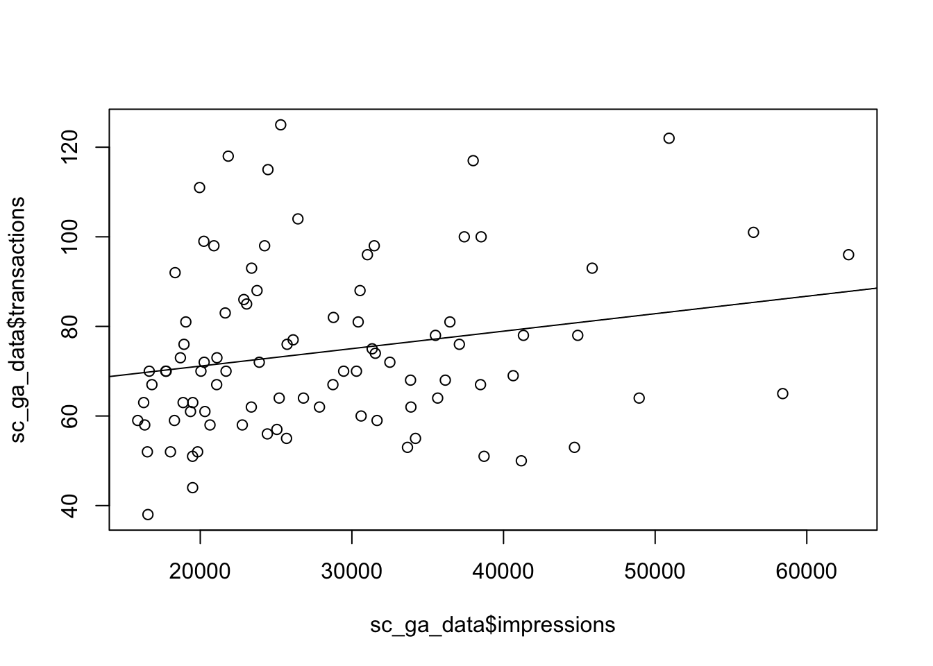
Multi-linear regression
Multi-linear regression is the same as simple linear regression, but you have more predictors - the below shows three (x, y, ø) with corresponding regression coefficients (A, B and C)
y = Ax + Bz + Cø + ePlotting a multi-linear regression is harder for more than 3 variables, as you need a multi-dimensional space, but its exactly the same principle - in this case the coefficients A, B and C show how much y would change if their respective regressor changed by 1 (and everything else stayed the same)
In R, you create multi-linear regression via the lm() function again, but you just add more variables to the model formula:
model2 <- lm(transactions ~ impressions + sessions + position, data = sc_ga_data)
## overall model statistics
glance(model2)
## r.squared adj.r.squared sigma statistic p.value df logLik
## 1 0.1642764 0.1351233 17.43101 5.634947 0.001421253 4 -382.9012
## AIC BIC deviance df.residual
## 1 775.8025 788.3015 26130.25 86## coefficients
tidy(model2)## term estimate std.error statistic p.value
## 1 (Intercept) 69.8256229916 2.997209e+01 2.3296885 0.02216593
## 2 impressions -0.0001550714 2.905029e-04 -0.5338034 0.59485465
## 3 sessions 0.0394295484 1.331140e-02 2.9620894 0.00395002
## 4 position -1.3288129470 1.161496e+00 -1.1440533 0.25577588The \(R^2\) value has improved a little so we can explain 16% of transactions from our model.
How do you think the coefficients of multiple linear regression applied to all Google Analytics sessions compare to the actual conversion rate registered in the E-commerce reports? What about the multi-touch reports?
Logit (Logistic) regression
Instead of a metric dependent variable, a binary (e.g., yes/no, on/off) dependent variable can be use. For example, the digital analyst would ask, “Did you open the email?” or “Did you visit the webpage?” The responses are binary. Using logit regression, the model can predict the probability that a person would be in the yes group or the no group.
In R, you create logistic regression by using the glm() function and passing in a family argument. In this case we choose binomial (another name for logistic), but the argument takes many other names too for different types of regression - see ?family for details.
model <- glm(sale ~ saw.promotion + existing.customer + hour.of.day,
             data = webdata,
             family = binomial)
Tobit Regression
This form of regression is an extension of logit regression.
Lemdep (limited dependent) regression
If the dependent variable has a ceiling (i.e., top code) or a floor (i.e., bottom code), then technically lemdep (or limited dependent) regression should be used. Ceilings and/or floors in the dependent variable relate to capacity constraints. For example, a live feed streaming from a website could only allow 1,000 active streams. If we want to predict the likelihood that a person will stream our content, then we need to use lemdep because the dependent variable (in this examples, number of active streams) appears top coded.
Summary
Regression is the only analytical tool that allows for prediction. To perform a regression analysis, the digital analyst needs to include at least one metric independent variable and one metric dependent variable.
The adjusted R Square expalins the amount of variance in the dependent variable explained by the inclusion of the independent variable. The unstandardized B generate the desired prediction line. The standardize B allow for a comparison of the independent variables to determine those variables that provide insight and those variables that are superfluous.
This section is intended to introduce regression. There is enough here to get even a beginning digital analyst started.