Advanced Dynamic Segments with ganalytics
This example demonstrates another way of defining dynamic segments by using functions from the ganalytics package. As of the most recent update to this site, this requires a “dev” (development) version of two packages (both packages exist on CRAN, but they require the dev versions to use the examples here):
googleAnalyticsRganalytics
This actually means this example has the incidental educational value of showing how to use packages from GitHub! You can read up on the purpose of ganalytics – developed by Johann de Boer – on GitHub. But, in short, it’s intended to “support R users in defining reporting queries using natural R expressions instead of being concerned about API technical intricacies like query syntax, character code escaping and API limitations.”
Setup/Config
This example requires development versions of the googleAnalyticsR (>=0.5.0.9000) and ganalytics (>=0.10.4.9000) R packages available on GitHub, so the setup code below is a bit different (it has some additional code for loading a couple of packages from GitHub).
Be sure you’ve completed the steps on the Initial Setup page before running this code.
For the setup, we’re going to load a few libraries, load our specific Google Analytics credentials, and then authorize with Google.
# Load the necessary libraries. These libraries aren't all necessarily required for every
# example, but, for simplicity's sake, we're going ahead and including them in every example.
# The "typical" way to load these is simply with "library([package name])." But, the handy
# thing about using the approach below -- which uses the pacman package -- is that it will
# check that each package exists and actually install any that are missing before loading
# the package.
if (!require("pacman")) install.packages("pacman")
pacman::p_load(tidyverse,         # Includes dplyr, ggplot2, and others; very key!
               devtools,          # Generally handy
               googleVis,         # Useful for some of the visualizations
               scales)            # Useful for some number formatting in the visualizations

# A function to check that a sufficiently current version of a specific package is
# installed and loaded. This isn't particularly elegant, but it works.
package_check <- function(package, min_version, github_location){
  # Check if ANY version of the package is installed. This is clunky, but p_load_current_gh
  # wasn't playing nice (and this does need some conditional checking.)
  if(package %in% rownames(installed.packages())){
    # IF a version of the package is already installed, then check the *version* of that
    # package to make sure it's current enough. If it'snot, then re-install from GitHub
    if(packageVersion(package) < min_version) {
      devtools::install_github(github_location)
    }
  } else {
    devtools::install_github(github_location)
  }
  # Load the package
  library(package, character.only = TRUE)
}

# As needed, install and load googleAnalyticsR and ganalytics from GitHub
package_check("googleAnalyticsR", "0.5.0.9001", "MarkEdmondson1234/googleAnalyticsR")
package_check("ganalytics", "0.10.4.9000", "jdeboer/ganalytics")

# Authorize GA. Depending on if you've done this already and a .ga-httr-oauth file has
# been saved or not, this may pop you over to a browser to authenticate.
ga_auth(token = ".ga-httr-oauth")

# Set the view ID and the date range. If you want to, you can swap out the Sys.getenv()
# call and just replace that with a hardcoded value for the view ID. And, the start
# and end date are currently set to choose the last 30 days, but those can be
# hardcoded as well.
view_id <- Sys.getenv("GA_VIEW_ID")
start_date <- Sys.Date() - 31        # 30 days back from yesterday
end_date <- Sys.Date() - 1           # Yesterday
If that all runs with just some messages but no errors, then you’re set for the next chunk of code: pulling the data.
Pull the Data
In this example, we’ll define a list of six segments dynamically, pull the total users and sessions for each segment, and then combine those results into a single data frame that we can view and visualize.
We’ll use ganalytics expressions (using the Expr() function) to define the criteria for each segment. Then, we’ll combine those into a list that, ultimately, we will work on to actually pull the data.
# Bounced sessions: Sessions where the bounces metric is not zero. The base "bounces" expression gets
# used in a couple of ways. For the "bounced users," it get passed to the PerSession() function to
# only count once per session
bounces <- Expr(~bounces != 0)
bounced_sessions <- PerSession(bounces)

# Mobile or tablet sessions: Sessions by mobile and tablet users.
mobile_or_tablet <- Expr(~deviceCategory %in% c("mobile", "tablet"))

# Converters: Users who performed any type of conversion during the defined date range. Note
# how the base expression is then passed into the PerUser() function to get a "per user" count
# of converters.
conversions <- Expr(~goalCompletionsAll > 0) | Expr(~transactions > 0)
converters <-  PerUser(conversions)

# Multi-session users: Users who have visited more than once during the defined date range.
# This uses both PerUser() and Include() to properly calculate mutiple sessions
multi_session_users <- Expr(~sessions > 1) %>% PerUser() %>% Include(scope = "users")

# New desktop users: Sessions by new visitors using a desktop device.
new_desktop_users <- Expr(~deviceCategory == "desktop") & Expr(~userType == "new")

# Bounced before converting = Users who bounced in one session before converting later.
bounced_before_converting <- Sequence(bounces, conversions, scope = "users")

# Now, combine all of these into a single list so we can work with it as one object
my_segment_list <- list(
  bounced_sessions = bounced_sessions,
  mobile_or_tablet = mobile_or_tablet,
  converters = converters,
  multi_session_users = multi_session_users,
  new_desktop_users = new_desktop_users,
  bounced_before_converting = bounced_before_converting
)
Because the Google Analytics Reporting API can only be used to query 4 segments at a time, we need to break our list segments into chunks before using googleAnalyticsR to query each chunk of segments and bind the results into a single data.frame. For each segment, we will request a count of users and sessions.
# Split our list into chunks with no more than four segments in each chunk
segment_chunks <- split(my_segment_list, (seq_along(my_segment_list) - 1L) %/% 4L)

# Pull the data. map_df will ensure the results are returned in a data frame.
results <- map_df(segment_chunks, function(chunk) {
  google_analytics(
    viewId = view_id,
    date_range = c(start_date, end_date),
    metrics = c("users", "sessions"),
    dimensions = c("segment"),
    segments = Segments(chunk)
  )
})

# Display the results
results| segment | users | sessions |
|---|---|---|
| bounced_sessions | 3283 | 4340 |
| converters | 15 | 36 |
| mobile_or_tablet | 618 | 909 |
| multi_session_users | 313 | 897 |
| bounced_before_converting | 3 | 17 |
| new_desktop_users | 3418 | 3543 |
Data Munging
We will compare users and sessions for each segment using a horizontal column chart. To do this we need to transform the results table into long format in which the count of users and sessions for each segment are on separate rows.
results_long <- results %>%
  gather(metric, count, users, sessions)

# Display the results
results_long| segment | metric | count |
|---|---|---|
| bounced_sessions | users | 3283 |
| converters | users | 15 |
| mobile_or_tablet | users | 618 |
| multi_session_users | users | 313 |
| bounced_before_converting | users | 3 |
| new_desktop_users | users | 3418 |
| bounced_sessions | sessions | 4340 |
| converters | sessions | 36 |
| mobile_or_tablet | sessions | 909 |
| multi_session_users | sessions | 897 |
| bounced_before_converting | sessions | 17 |
| new_desktop_users | sessions | 3543 |
Data Visualization
Finally, create a horizontal bar chart showing the results.
# Create the plot. Note the stat="identity"" (because the data is already aggregated) and
# the coord_flip(). And, I just can't stand it... added on the additional theme stuff to
# clean up the plot a bit more.
gg <- ggplot(results_long) +
  aes(segment, count, fill = metric) +
  geom_col(position = "dodge") +
  coord_flip() +
  guides(fill = guide_legend(reverse = TRUE)) +
  theme_light()

# Output the plot. You *could* just remove the "gg <-" in the code above, but it's
# generally a best practice to create a plot object and then output it, rather than
# outputting it on the fly.
gg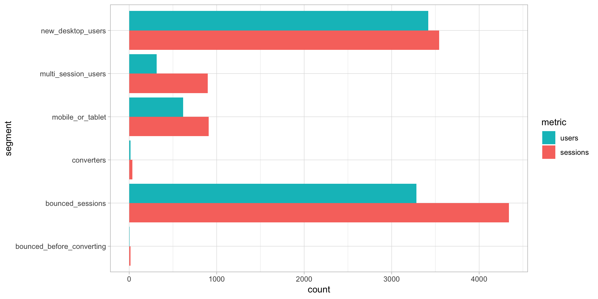
This site is a sub-site to dartistics.com