Simple Dynamic Segment - v4
This example pulls the top 10 pages for the last thirty days, for visits that occurred on a mobile device. For the sake of illustration, we’re going to build this segment dynamically rather than referencing a segment ID. Where this can come in handy is if you have a script where you want to work through a range of small little tweaks to one segment and re-pull the data. You don’t want to build each segment in the web interface and then hardcode all those IDs! We may add an example for doing that later, but we’re doing to keep this very simple for now.
This returns the exact same results as these two examples, but through different means for defining/referencing the segment:
- Simple Dynamic Segment - v3 – Ahhhhh! The days when dynamic segments were so much simpler (but also less powerful)
- Apply Segment by Segment ID – simply using the ID of either a standard segment or a custom segment built in the Google Analytics web interface
With the v4 API, dynamic segments are more powerful than v3, but (alas!) pretty basic segments can feel pretty convoluted.
Setup/Config
Be sure you’ve completed the steps on the Initial Setup page before running this code.
For the setup, we’re going to load a few libraries, load our specific Google Analytics credentials, and then authorize with Google.
# Load the necessary libraries. These libraries aren't all necessarily required for every
# example, but, for simplicity's sake, we're going ahead and including them in every example.
# The "typical" way to load these is simply with "library([package name])." But, the handy
# thing about using the approach below -- which uses the pacman package -- is that it will
# check that each package exists and actually install any that are missing before loading
# the package.
if (!require("pacman")) install.packages("pacman")
pacman::p_load(googleAnalyticsR,  # How we actually get the Google Analytics data
               tidyverse,         # Includes dplyr, ggplot2, and others; very key!
               devtools,          # Generally handy
               googleVis,         # Useful for some of the visualizations
               scales)            # Useful for some number formatting in the visualizations

# Authorize GA. Depending on if you've done this already and a .ga-httr-oauth file has
# been saved or not, this may pop you over to a browser to authenticate.
ga_auth(token = ".ga-httr-oauth")

# Set the view ID and the date range. If you want to, you can swap out the Sys.getenv()
# call and just replace that with a hardcoded value for the view ID. And, the start
# and end date are currently set to choose the last 30 days, but those can be
# hardcoded as well.
view_id <- Sys.getenv("GA_VIEW_ID")
start_date <- Sys.Date() - 31        # 30 days back from yesterday
end_date <- Sys.Date() - 1           # Yesterday
If that all runs with just some messages but no errors, then you’re set for the next chunk of code: pulling the data.
Pull the Data
This all gets built up in what can feel very cumbersome. Check out ?segment_ga4() for the documentation of how the segment gets built. Correctly, it describes this as a “hierarchy.” In practical terms, though, we build from the bottom up:
- Define a segment element using
segment_element(). This is just a single conditional statement. - Combine one or more segment elements together into a segment vector using
segment_vector_simple(). There are a few options here, but we’re going to stick with the simple approach. And, it’s still going to feel redundant, because we’re only including a single segment element. - Combine one or more segment vectors into a segment definition using
segment_define(). This may feel like it’s the same as the previous step, but, if you think about the segment builder in the web interface, it will start to make sense – there are two levels at which can combine multiple “things” together to define a segment. Alas! Here, again, we’re just including a single segment vector, so it all feels really cumbersome. - Put that into a segment object, which is what we’re actually going to use in the data. We actually give the segment a name here that will be returned in the results.
- Actually pull the data, passing in the segment object as an argument.
In addition to the “hierarchy” messiness for a simple segment, there is also some list() messiness. Note, for instance, how my_segment_vector in the example code includes a list within a list. Use this example (and other examples on this site) as well as the ?segment_ga4() documentation to troubleshoot.
# Create a segment element object. See ?segment_element() for details.
my_segment_element <- segment_element("deviceCategory",
                                   operator = "EXACT",
                                   type = "DIMENSION",
                                   expressions = "Mobile")

# Create a segment vector that has just one element. See ?segment_vector_simple() for details. Note
# that the element is wrapped in a list(). This is how you would include multiple elements in the
# definition.
my_segment_vector <- segment_vector_simple(list(list(my_segment_element)))

# Define the segment with just the one segment vector in it. See ?segment_define() for details.
my_segment_definition <- segment_define(list(my_segment_vector))

# Create the actual segment object that we're going to use in the query. See ?segment_ga4()
# for details.
my_segment <- segment_ga4("Mobile Sessions Only",
                                 session_segment = my_segment_definition)

# <whew>!!!

# Pull the data. See ?google_analytics_4() for additional parameters. Depending on what
# you're expecting back, you probably would want to use an "order" argument to get the
# results in descending order. But, we're keeping this example simple. Note, though, that
# we're still wrapping my_segment in a list() (of one element).
ga_data <- google_analytics(viewId = view_id,
                              date_range = c(start_date, end_date),
                              metrics = "pageviews",
                              dimensions = "pagePath",
                              segments = my_segment)

# Go ahead and do a quick inspection of the data that was returned. This isn't required,
# but it's a good check along the way.
head(ga_data)| pagePath | segment | pageviews |
|---|---|---|
| / | Mobile Sessions Only | 269 |
| /?__hstc=205162639.2492ee4e2514a59ed226f9dc5224e8b6.1537248787762.1537248787762.1537248787762.1&__hssc=205162639.1.1537248787763&__hsfp=2964561211&hsCtaTracking=8bc9e3c4-0d81-453f-9aa0-e7ee2d150e86|4361a058-c61b-4634-98be-95a3d7d9cb0c | Mobile Sessions Only | 1 |
| /?__hstc=205162639.3ee49b04f9a3ca95eff26980d8739ac8.1537165640249.1537165640249.1537165640249.1&__hssc=&hsCtaTracking=8bc9e3c4-0d81-453f-9aa0-e7ee2d150e86|4361a058-c61b-4634-98be-95a3d7d9cb0c | Mobile Sessions Only | 1 |
| /about/ | Mobile Sessions Only | 43 |
| /about/career-spotlights/ | Mobile Sessions Only | 1 |
| /about/careers/ | Mobile Sessions Only | 83 |
Data Munging
Since we didn’t sort the data when we queried it, let’s go ahead and sort it here and grab just the top 10 pages.
# Using dplyr, sort descending and then grab the top 10 values. We also need to make the
# page column a factor so that the order will be what we want when we chart the data.
# This is a nuisance, but you get used to it. That's what the mutate function is doing.
ga_data_top_10 <- ga_data %>%
  arrange(-pageviews) %>%
  top_n(10) %>%
  mutate(pagePath = factor(pagePath,
                           levels = rev(pagePath)))

# Take a quick look at the result.
head(ga_data_top_10)| pagePath | segment | pageviews |
|---|---|---|
| / | Mobile Sessions Only | 269 |
| /open-positions/ | Mobile Sessions Only | 124 |
| /about/careers/ | Mobile Sessions Only | 83 |
| /solutions/industries/ | Mobile Sessions Only | 49 |
| /solutions/partners/adobe/adobe-launch/dtm-launch-assessment/ | Mobile Sessions Only | 48 |
| /about/ | Mobile Sessions Only | 43 |
Data Visualization
This won’t be the prettiest bar chart, but let’s make a horizontal bar chart with the data. Remember, in ggplot2, a horizontal bar chart is just a normal bar chart with coord_flip().
# Create the plot. Note the stat="identity"" (because the data is already aggregated) and
# the coord_flip(). And, I just can't stand it... added on the additional theme stuff to
# clean up the plot a bit more.
gg <- ggplot(ga_data_top_10, mapping = aes(x = pagePath, y = pageviews)) +
  geom_bar(stat = "identity") +
  coord_flip() +
  theme_light() +
  theme(panel.grid.major.y = element_blank(),
        panel.grid.minor.y = element_blank(),
        panel.border = element_blank(),
        axis.title.y = element_blank(),
        axis.ticks.y = element_blank())

# Output the plot. You *could* just remove the "gg <-" in the code above, but it's
# generally a best practice to create a plot object and then output it, rather than
# outputting it on the fly.
gg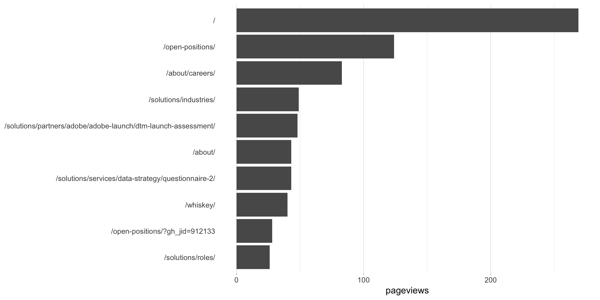
This site is a sub-site to dartistics.com