Traffic by Device Category
This example pulls sessions and by device category for the last 30 days and then plots the data on a line chart.
Setup/Config
Be sure you’ve completed the steps on the Initial Setup page before running this code.
For the setup, we’re going to load a few libraries, load our specific Google Analytics credentials, and then authorize with Google.
# Load the necessary libraries. These libraries aren't all necessarily required for every
# example, but, for simplicity's sake, we're going ahead and including them in every example.
# The "typical" way to load these is simply with "library([package name])." But, the handy
# thing about using the approach below -- which uses the pacman package -- is that it will
# check that each package exists and actually install any that are missing before loading
# the package.
if (!require("pacman")) install.packages("pacman")
pacman::p_load(googleAnalyticsR,  # How we actually get the Google Analytics data
               tidyverse,         # Includes dplyr, ggplot2, and others; very key!
               devtools,          # Generally handy
               googleVis,         # Useful for some of the visualizations
               scales)            # Useful for some number formatting in the visualizations

# Authorize GA. Depending on if you've done this already and a .ga-httr-oauth file has
# been saved or not, this may pop you over to a browser to authenticate.
ga_auth(token = ".ga-httr-oauth")

# Set the view ID and the date range. If you want to, you can swap out the Sys.getenv()
# call and just replace that with a hardcoded value for the view ID. And, the start
# and end date are currently set to choose the last 30 days, but those can be
# hardcoded as well.
view_id <- Sys.getenv("GA_VIEW_ID")
start_date <- Sys.Date() - 31        # 30 days back from yesterday
end_date <- Sys.Date() - 1           # Yesterday
If that all runs with just some messages but no errors, then you’re set for the next chunk of code: pulling the data.
Pull the Data
This is a simple query.
# Pull the data. See ?google_analytics_4() for additional parameters. The anti_sample = TRUE
# parameter will slow the query down a smidge and isn't strictly necessary, but it will
# ensure you do not get sampled data.
ga_data <- google_analytics(viewId = view_id,
                              date_range = c(start_date, end_date),
                              metrics = "sessions",
                              dimensions = c("date","deviceCategory"),
                              anti_sample = TRUE)

# Go ahead and do a quick inspection of the data that was returned. This isn't required,
# but it's a good check along the way.
head(ga_data)| date | deviceCategory | sessions |
|---|---|---|
| 2018-09-10 | desktop | 160 |
| 2018-09-10 | mobile | 15 |
| 2018-09-10 | tablet | 4 |
| 2018-09-11 | desktop | 217 |
| 2018-09-11 | mobile | 50 |
| 2018-09-11 | tablet | 1 |
Data Munging
We don’t actually need to do any data munging in this example (although, in practice, there may be some cleanup that you’d wind up wanting to do). The data as it comes out of GA is pretty much plottable as is.
Data Visualization
This won’t be the prettiest plot, but this example isn’t diving into the details of ggplot2. If you want to read up on that, this page on dartistics.com is worth checking out.
# Create the plot.
gg <- ggplot(ga_data, mapping = aes(x = date, y = sessions, colour = deviceCategory)) +
  geom_line() +
  theme_light()

# Output the plot. You *could* just remove the "gg <-" in the code above, but it's
# generally a best practice to create a plot object and then output it, rather than
# outputting it on the fly.
gg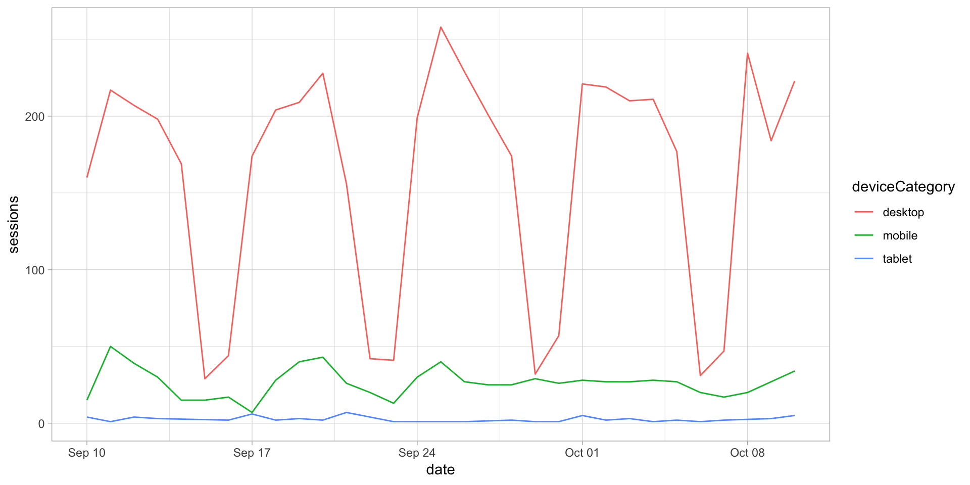
This site is a sub-site to dartistics.com