RMarkdown

What is (R)Markdown?

“Markdown” is “lightweight” markup language (yeah… markdown is markup…). HTML is HyperText Markup Language designed specifically for delivering web pages. Mark_down_, generically, is much simpler, and it’s not wedded to any particular output format.

“RMarkdown” is the R-specific version of markdown. It isn’t infinitely flexible, but it’s still quite rich in what it can render as output. At it’s core, though, it’s just a text file that uses a specific syntax.

Once you pivot to a specific output format – PDF, HTML, MS Word, slides, books, websites (like this one) – you can start to further extend the formatting options. Sometimes that comes with some complexity, but it’s all generally pretty manageable.

.R? Nope. .Rmd!

R scripts (typically) have a .R file extension. RMarkdown files, instead, have a .Rmd extension. When you create an RMarkdown file (File >> New File >> RMarkdown…) the script editor will have some additional options at the top of it.

The top of the script editor in RStudio looks like this if you’re editing an R script:

Contrast that with what it looks like when you open a .Rmd file:

What is Knit?! Well, we “Source” R scripts to execute an entire file. We “Knit” RMarkdown files. Basically, that just means a separate engine goes through the file, converts it to “true” markdown, executes any code embedded in the file, generates output from that code, and then builds the final output.

This web page, for instance, is a file called basic-rmarkdown.Rmd. Whenever we knit it, it generates a file called basic-rmarkdown.html, which is the actual file you are viewing right now.

Basic Formatting

There are some great and easily accessible resources for getting the basics of formatting with RMarkdown. http://rmarkdown.rstudio.com is an easy-to-use reference, but so are the links available from the Help menu inside RStudio:

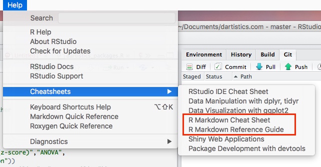
Take a minute to check out the **R Markdown Reference Guide to see how #, _, *, and [] get put to use to indicate heading styles, bold and italicized text, bullets, links, and images. It’s an easy “language” to learn!

Inserting Code

Simply being able to insert and style text and images isn’t the real power of RMarkdown. The real power comes from embedding code in the file. Think of a weekly report that you need to compile. You can use the Sys.Date() function to dynamically determine the start and end dates for the data in the report, and then, every time the .Rmd file gets “knitted,” the data that it uses will dynamically update to the most appropriate timeframe.

Exercise: Make Some Slides

In this exercise, we’re going to create a simple set of slides and put some very simple code in them:

1. Select File>>New File>>RMarkdown
2. Select Presentation and HTML (ioslides)
3. Give the presentation a name like “My First RMarkdown.” You should now have a shell RMarkdown document.
4. Go ahead and click Knit. You will be prompted to save the file first, so go ahead and do that. The result will be a simple 5-slide deck.
5. Go ahead and close the window with the presentation.
6. Delete the “Slide with bullets” slide (the ## serves as both a “Heading 2” and, in this case, as the indicator that it is a new slide)
7. Add a new slide after the R Markdown slide with a title of “Today’s Date”
8. For this slide, we’ll do full R Code, so place the cursor below the title and click the Insert button and select R to generate the RMarkdown syntax for embedding R code. This syntax is so simple that it’s almost faster to just type it!
9. For the code – inside the gray area – simply type Sys.Date()
10. Knit the presentation and check out the slide. It’s not pretty, but it’s displaying the results of a function!
11. Go back into the editor and add inline code. On the same slide, but after the closing ```’s, enter Put more cleanly, today is, then insert a single backtick, the letter “r”, Sys.Date(), and then another single backtick.
12. Knit the presentation again.

Extra credit: Create a new slide that uses the ggplot code we created earlier!

That’s the basics of RMarkdown. There is a lot more to it – a LOT – but we’ll cover that in the Advanced RMarkdown section!

A Few More Notes

A few handy tips:

• Inside curly braces where you initiate a block of R code, there are two things you can add:
  • A name for the snippet. This can be handy for troubleshooting where the knitting process is breaking (but, if a snippet has a name, it has to be unique across all snippets in the file)
  • You can add parameters like echo, include, eval, and warnings and more to control which aspects of the underlying code actually get displayed and/or executed. Read more about those here and here.
• When you knit an entire document, nothing shows up in your Environment. That can make it pesky to troubleshoot. But, just like any R script, you can execute a single line of code in a code snippet by placing your cursor in the line and pressing <Ctrl>-<Enter>. You can highlight multiple lines of code and press <Ctrl>-<Enter> to execute all of those lines. And, you can select Run>>Run Current Chunk or press <Ctrl>-Shift-<Enter> to run the current chunk of code. This will both generate the results (if there are any) inline and will create any objects in the Environment for you to inspect (or further manipulate).
• It can sometimes be easier to initially write the code as a .R script and then bring it into a .Rmd file once you have the guts of the code working.